UTS#

Lakukan analisa terhadap data pada https://archive.ics.uci.edu/ml/datasets/Breast+Cancer+Coimbra dengan menggunakan klasifikasi

metode KNN
metode pohon keputusan (Desision tree)

Proses analisa dilaporkan dan diupload di github ( menggunakan jupyter book)

Metode KNN#

Connect to google drive
Import Library

import pandas as pd
import numpy as np
import seaborn as sns 
import matplotlib.pyplot as plt

Ambil data

%cd /content/drive/MyDrive/datamining/tugas/data/

/content/drive/MyDrive/datamining/tugas/data

data = pd.read_csv("dataR2.csv")
data.head()

	Age	BMI	Glucose	Insulin	HOMA	Leptin	Adiponectin	Resistin	MCP.1	Classification
0	48	23.500000	70	2.707	0.467409	8.8071	9.702400	7.99585	417.114	1
1	83	20.690495	92	3.115	0.706897	8.8438	5.429285	4.06405	468.786	1
2	82	23.124670	91	4.498	1.009651	17.9393	22.432040	9.27715	554.697	1
3	68	21.367521	77	3.226	0.612725	9.8827	7.169560	12.76600	928.220	1
4	86	21.111111	92	3.549	0.805386	6.6994	4.819240	10.57635	773.920	1

Cek dataset

data

	Age	BMI	Glucose	Insulin	HOMA	Leptin	Adiponectin	Resistin	MCP.1	Classification
0	48	23.500000	70	2.707	0.467409	8.8071	9.702400	7.99585	417.114	1
1	83	20.690495	92	3.115	0.706897	8.8438	5.429285	4.06405	468.786	1
2	82	23.124670	91	4.498	1.009651	17.9393	22.432040	9.27715	554.697	1
3	68	21.367521	77	3.226	0.612725	9.8827	7.169560	12.76600	928.220	1
4	86	21.111111	92	3.549	0.805386	6.6994	4.819240	10.57635	773.920	1
...	...	...	...	...	...	...	...	...	...	...
111	45	26.850000	92	3.330	0.755688	54.6800	12.100000	10.96000	268.230	2
112	62	26.840000	100	4.530	1.117400	12.4500	21.420000	7.32000	330.160	2
113	65	32.050000	97	5.730	1.370998	61.4800	22.540000	10.33000	314.050	2
114	72	25.590000	82	2.820	0.570392	24.9600	33.750000	3.27000	392.460	2
115	86	27.180000	138	19.910	6.777364	90.2800	14.110000	4.35000	90.090	2

116 rows × 10 columns

print(len(data),len(data.columns))

116 10

Exploratory data analysis

data.info()

<class 'pandas.core.frame.DataFrame'>
RangeIndex: 116 entries, 0 to 115
Data columns (total 10 columns):
 #   Column          Non-Null Count  Dtype  
---  ------          --------------  -----  
 0   Age             116 non-null    int64  
 1   BMI             116 non-null    float64
 2   Glucose         116 non-null    int64  
 3   Insulin         116 non-null    float64
 4   HOMA            116 non-null    float64
 5   Leptin          116 non-null    float64
 6   Adiponectin     116 non-null    float64
 7   Resistin        116 non-null    float64
 8   MCP.1           116 non-null    float64
 9   Classification  116 non-null    int64  
dtypes: float64(7), int64(3)
memory usage: 9.2 KB

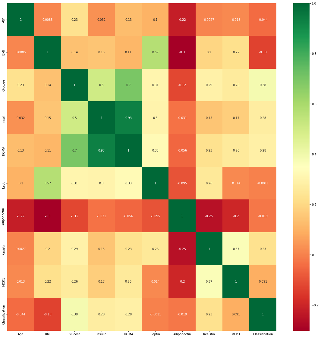
Visualisasi correlation grid

plt.subplots(figsize=(20,20))
sns.heatmap(data.corr(),cmap='RdYlGn',annot=True)

<matplotlib.axes._subplots.AxesSubplot at 0x7f46426c4e10>

# create the features from data
X=data.iloc[:,0:9]

# create the target variable from data
Y=data.iloc[:,9]

X.head()

	Age	BMI	Glucose	Insulin	HOMA	Leptin	Adiponectin	Resistin	MCP.1
0	48	23.500000	70	2.707	0.467409	8.8071	9.702400	7.99585	417.114
1	83	20.690495	92	3.115	0.706897	8.8438	5.429285	4.06405	468.786
2	82	23.124670	91	4.498	1.009651	17.9393	22.432040	9.27715	554.697
3	68	21.367521	77	3.226	0.612725	9.8827	7.169560	12.76600	928.220
4	86	21.111111	92	3.549	0.805386	6.6994	4.819240	10.57635	773.920

Y.head()

  1
  1
  1
  1
  1
Name: Classification, dtype: int64

Menggunakan Standardisasi untuk membawa semua nilai ke satu unit karena KNN adalah metode berbasis jarak

from sklearn.preprocessing import StandardScaler
ss=StandardScaler()
X=ss.fit_transform(X)
X=pd.DataFrame(X)

Splitting of Dataset untuk uji

from sklearn.model_selection import train_test_split
xtrain,xtest,ytrain,ytest=train_test_split(X,Y,test_size=0.3)

Membangun classifier KNeighbors menggunakan simulasi nilai k yang berbeda

#Importing KNeighbors Classifier from sklearn
#Finding accuracies  on TrainData and Test data with euclidean distance(by default p=2)
from sklearn.neighbors import KNeighborsClassifier
from sklearn.metrics import accuracy_score
for x in range(5,10,2):
    knn=KNeighborsClassifier(n_neighbors=x,metric='minkowski',weights='distance')
    knn.fit(xtrain,ytrain)
    train_ypred=knn.predict(xtrain)
    acc_train_score=accuracy_score(train_ypred,ytrain)
    test_ypred=knn.predict(xtest)
    acc_test_score=accuracy_score(test_ypred,ytest)
    print(f'Skor akurasi untuk data uji adalah {acc_train_score} and {acc_test_score} untuk {x} neighbours')

Skor akurasi untuk data uji adalah 1.0 and 0.8285714285714286 untuk 5 neighbours
Skor akurasi untuk data uji adalah 1.0 and 0.7714285714285715 untuk 7 neighbours
Skor akurasi untuk data uji adalah 1.0 and 0.6857142857142857 untuk 9 neighbours

Membangun classifier KNeighbors menggunakan Eucledian Distance dan 7 neighbours

knn=KNeighborsClassifier(n_neighbors=7,metric='minkowski',weights='distance')
knn.fit(xtrain,ytrain)

KNeighborsClassifier(n_neighbors=7, weights='distance')

# Predicting for train data
trainypred=knn.predict(xtrain)

Finding the precision, recall, f1-score ,support

# Classification report on train data set
from sklearn.metrics import classification_report
print(classification_report(trainypred,ytrain))

              precision    recall  f1-score   support

           1       1.00      1.00      1.00        36
           2       1.00      1.00      1.00        45

    accuracy                           1.00        81
   macro avg       1.00      1.00      1.00        81
weighted avg       1.00      1.00      1.00        81

# Mencari skor akurasi
accuracy_score(trainypred,ytrain)

1.0

Memprediksi data tes

testypredicted=knn.predict(xtest)

# Skor akurasi data tes
from sklearn.metrics import accuracy_score
accuracy_score(testypredicted,ytest)

0.7714285714285715

Metode Decision Tree#

Classification

# classifying
from sklearn.tree import DecisionTreeClassifier
from sklearn.model_selection import train_test_split
from sklearn.metrics import accuracy_score
from io import StringIO


# pretty printing
from pprint import pprint

# visualizing 
import matplotlib.pyplot as plt
from IPython.display import Image  
from sklearn.tree import export_graphviz
import pydotplus

from sklearn.datasets import load_breast_cancer
data = load_breast_cancer()

# The shape of the data matrix (without class attribute)
print("Matrix shape: " + repr(data.data.shape))
# The names of the features
print("The data set has the following features:")
pprint(data.feature_names)
# The names of the classes
print("The data set has the following classes:")
pprint(data.target_names)

pprint(data.data[1])

# This prints a rather long descriptions.
# print(data.DESCR)

Matrix shape: (569, 30)
The data set has the following features:
array(['mean radius', 'mean texture', 'mean perimeter', 'mean area',
       'mean smoothness', 'mean compactness', 'mean concavity',
       'mean concave points', 'mean symmetry', 'mean fractal dimension',
       'radius error', 'texture error', 'perimeter error', 'area error',
       'smoothness error', 'compactness error', 'concavity error',
       'concave points error', 'symmetry error',
       'fractal dimension error', 'worst radius', 'worst texture',
       'worst perimeter', 'worst area', 'worst smoothness',
       'worst compactness', 'worst concavity', 'worst concave points',
       'worst symmetry', 'worst fractal dimension'], dtype='<U23')
The data set has the following classes:
array(['malignant', 'benign'], dtype='<U9')
array([2.057e+01, 1.777e+01, 1.329e+02, 1.326e+03, 8.474e-02, 7.864e-02,
       8.690e-02, 7.017e-02, 1.812e-01, 5.667e-02, 5.435e-01, 7.339e-01,
       3.398e+00, 7.408e+01, 5.225e-03, 1.308e-02, 1.860e-02, 1.340e-02,
       1.389e-02, 3.532e-03, 2.499e+01, 2.341e+01, 1.588e+02, 1.956e+03,
       1.238e-01, 1.866e-01, 2.416e-01, 1.860e-01, 2.750e-01, 8.902e-02])

# Split into training and test
X_train, X_test, y_train, y_test = train_test_split(data.data[:,0:9],data.target,shuffle=True,test_size=0.3, random_state=42)

# DECISION TREE
# initialize the model with standard parameters
clf_dt = DecisionTreeClassifier(criterion="entropy")
# train the model
clf_dt.fit(X_train,y_train)

DecisionTreeClassifier(criterion='entropy')

# Evaluating on the test data
y_test_pred = clf_dt.predict(X_test);
a_dt_test = accuracy_score(y_test, y_test_pred);

# Evaluating on the training data
y_train_pred = clf_dt.predict(X_train);
a_dt_train = accuracy_score(y_train, y_train_pred);

print("Training data accuracy is " +  repr(a_dt_train) + " and test data accuracy is " + repr(a_dt_test))

Training data accuracy is 1.0 and test data accuracy is 0.9590643274853801

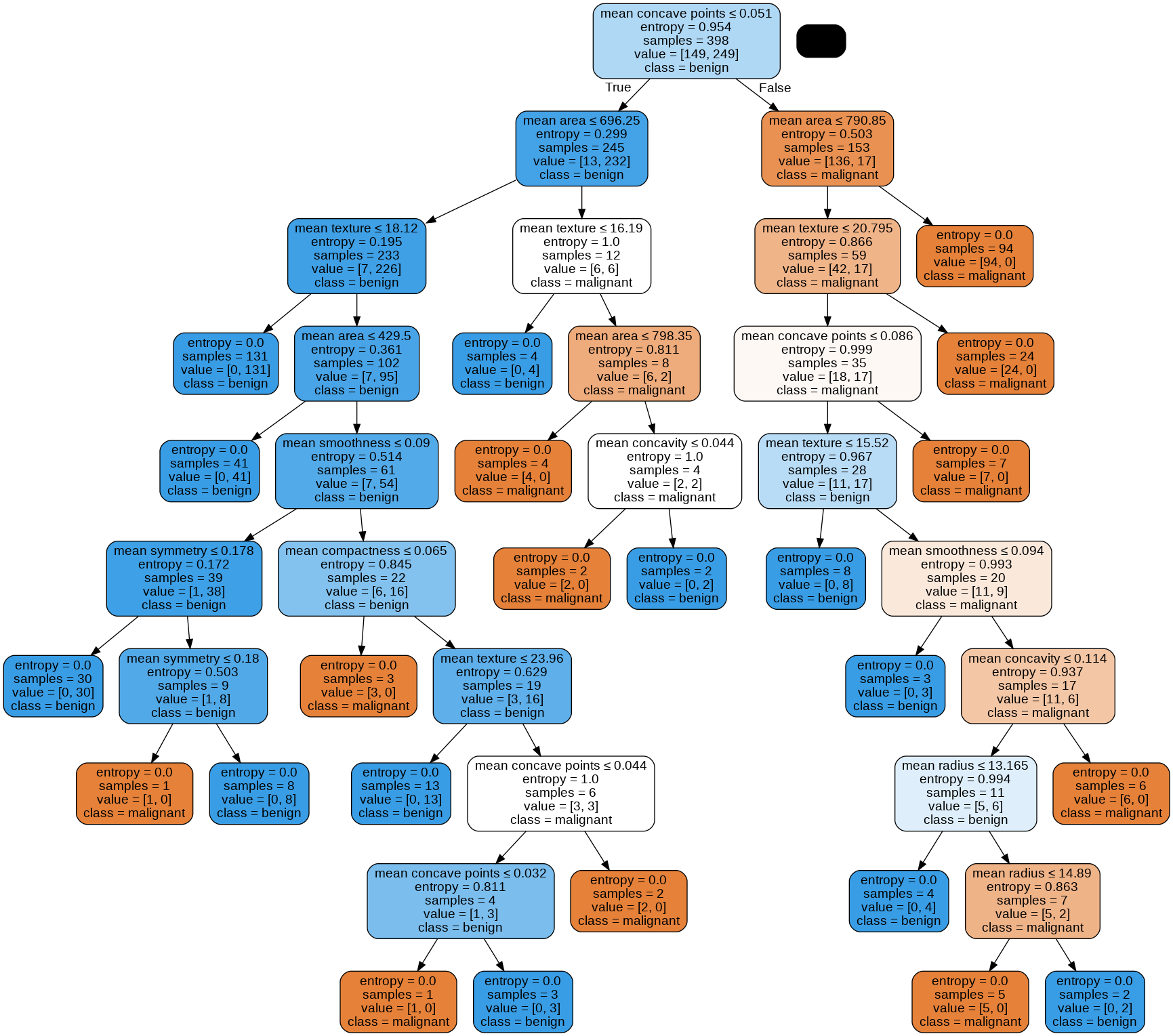
dot_data = StringIO()
export_graphviz(clf_dt, out_file=dot_data,
                feature_names=data.feature_names[0:9],  
                class_names=data.target_names,
                filled=True, rounded=True,
                special_characters=True)
graph = pydotplus.graph_from_dot_data(dot_data.getvalue())  
Image(graph.create_png())

My sample book

UTS

Contents

UTS#

Metode KNN#

Metode Decision Tree#