K-Means Clustering (Tugas 5)

Import Library

import numpy as np
import pandas as pd
import matplotlib.pyplot as plt
from sklearn import datasets
import seaborn as sns
from sklearn.cluster import KMeans

Ambil data

%cd /content/drive/MyDrive/datamining/tugas/Iris/

/content/drive/MyDrive/datamining/tugas/Iris

df = pd.read_csv("Iris.csv")
df.head()

	Id	SepalLengthCm	SepalWidthCm	PetalLengthCm	PetalWidthCm	Species
0	1	5.1	3.5	1.4	0.2	Iris-setosa
1	2	4.9	3.0	1.4	0.2	Iris-setosa
2	3	4.7	3.2	1.3	0.2	Iris-setosa
3	4	4.6	3.1	1.5	0.2	Iris-setosa
4	5	5.0	3.6	1.4	0.2	Iris-setosa

df.tail()

	Id	SepalLengthCm	SepalWidthCm	PetalLengthCm	PetalWidthCm	Species
145	146	6.7	3.0	5.2	2.3	Iris-virginica
146	147	6.3	2.5	5.0	1.9	Iris-virginica
147	148	6.5	3.0	5.2	2.0	Iris-virginica
148	149	6.2	3.4	5.4	2.3	Iris-virginica
149	150	5.9	3.0	5.1	1.8	Iris-virginica

data = df.drop(columns=['Id'])

Shape data

data.shape

(150, 5)

data.describe()

	SepalLengthCm	SepalWidthCm	PetalLengthCm	PetalWidthCm
count	150.000000	150.000000	150.000000	150.000000
mean	5.843333	3.054000	3.758667	1.198667
std	0.828066	0.433594	1.764420	0.763161
min	4.300000	2.000000	1.000000	0.100000
25%	5.100000	2.800000	1.600000	0.300000
50%	5.800000	3.000000	4.350000	1.300000
75%	6.400000	3.300000	5.100000	1.800000
max	7.900000	4.400000	6.900000	2.500000

Data Visualization

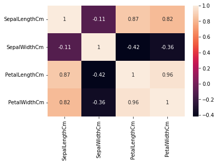
sns.heatmap(data.corr(), annot = True, linecolor='black')

<matplotlib.axes._subplots.AxesSubplot at 0x7fa688144190>

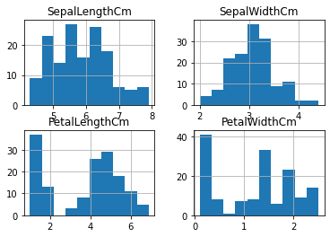
data.hist()
plt.show()

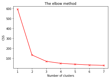
# Settin the data
x=data.iloc[:,0:3].values

css=[]

# Finding inertia on various k values
for i in range(1,8):
    kmeans=KMeans(n_clusters = i, init = 'k-means++', 
                    max_iter = 100, n_init = 10, random_state = 0).fit(x)
    css.append(kmeans.inertia_)
    
plt.plot(range(1, 8), css, 'bx-', color='red')
plt.title('The elbow method')
plt.xlabel('Number of clusters')
plt.ylabel('CSS') 
plt.show()

Applying K-Means Classifier

#Applying Kmeans classifier
kmeans = KMeans(n_clusters=3,init = 'k-means++', max_iter = 100, n_init = 10, random_state = 0)

y_kmeans = kmeans.fit_predict(x)

Visualizing the clusters

kmeans.cluster_centers_

array([[5.84655172, 2.73275862, 4.3637931 ],
       [5.006     , 3.418     , 1.464     ],
       [6.83571429, 3.06428571, 5.6547619 ]])

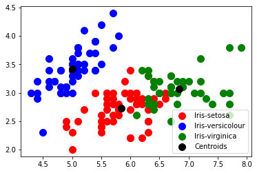
# Visualising the clusters - On the first two columns
plt.scatter(x[y_kmeans == 0, 0], x[y_kmeans == 0, 1], 
            s = 100, c = 'red', label = 'Iris-setosa')
plt.scatter(x[y_kmeans == 1, 0], x[y_kmeans == 1, 1], 
            s = 100, c = 'blue', label = 'Iris-versicolour')
plt.scatter(x[y_kmeans == 2, 0], x[y_kmeans == 2, 1],
            s = 100, c = 'green', label = 'Iris-virginica')

# Plotting the centroids of the clusters
plt.scatter(kmeans.cluster_centers_[:, 0], kmeans.cluster_centers_[:,1], 
            s = 100, c = 'black', label = 'Centroids')

plt.legend()

<matplotlib.legend.Legend at 0x7fa684e05990>